

2: Looking at the Results#
Introduction#
This tutorial will cover using the Dashboard, which you view in a Web browser, to examine the results of a job. It will show you how to see the text output from the job, look at the molecular structures, and also see the orbitals and charge densities.
Note
The present tutorial assumes you have read and followed the instructions laid out in 1: A First Calculation so that there is at least one job to work with.
Accessing the Dashboard#
By default, you can access the Dashboard at http://localhost:55055 (will open in a new tab):

The Dashboard when you first access it#
The left pane is a menu of various sections available in the Dashboard. The left arrow at the bottom-right part of this pane collapses the menu into icons adding more space for the right pane which may be useful in various situations e.g., when looking at the simulation outputs. The right pane presents a summary of the executed jobs, flowcharts and projects that the current user has the permission to view. On the first access to the Dashboard web-page, it shows everything with the public permission to anyone without logging in.
Let us begin by clicking on the Public User menu drop-down button at the upper-right
corner of the section and select Login or clicking on Log in in the blue
notification bar.
Note
When entering the username and password, remember that by default, the initial passwords for the admin and user accounts are set to admin and default, respectively. Hopefully, however, you went through the first tutorial and set up good passwords.
Once you are logged in, the front page of the Dashboard should change slightly and look like the following:
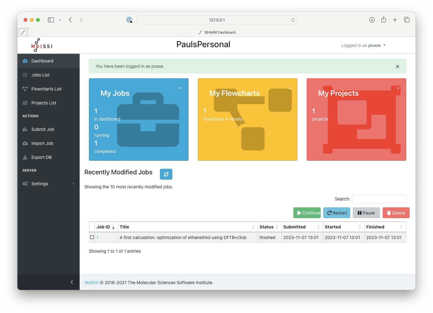
The Dashboard after logging in#
Note the summary of information regarding the executed jobs in the main colored card
sections: one job, one flowchart, and one project. You can use either the menu at the
top of each panel or the items in the left-pane menu in order to inspect jobs,
flowcharts, or projects. The bottom part of the main pane gives a short list of the most
recent jobs. We have only one, which you can access by clicking on the job number. More
generally, however, click on Jobs List in the left-pane menu to get a complete list
of jobs:
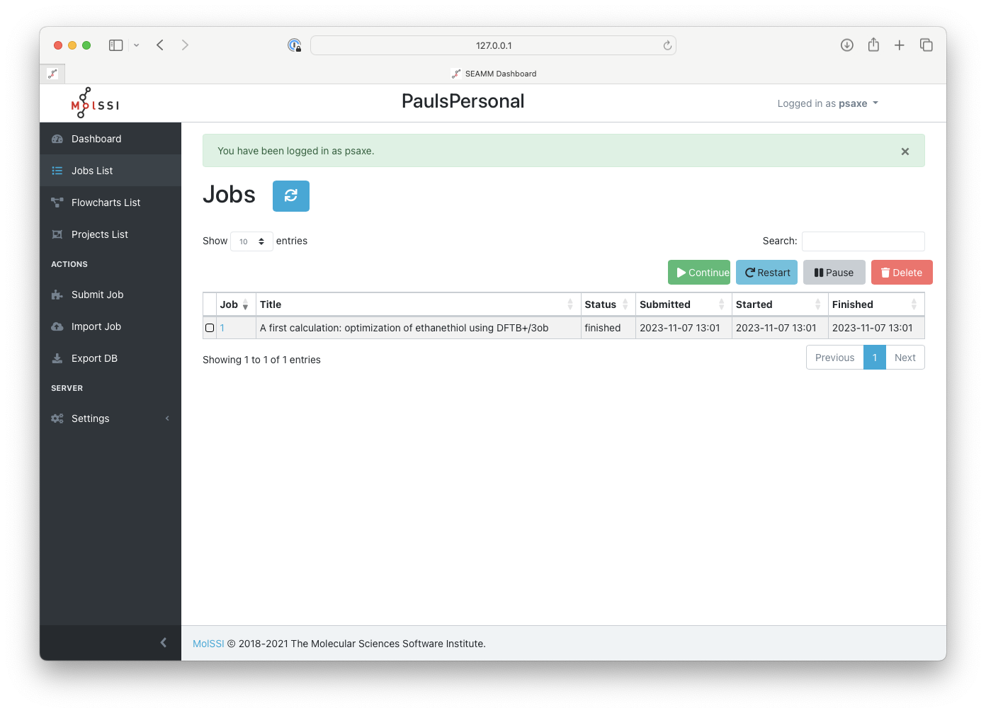
The list of jobs in the Dashboard#
Examining a Job#
If you just went through the tutorial for the first job, there is probably just one job in the list, as is shown.
Tip
The title that you give each job is important. You see the titles in the list of jobs, and can search on them, so it is a good idea to make them short but meaningful. They can only be 100 characters long, so a systematic approach with abbreviations works best.
Click on the job ID to expand its results:
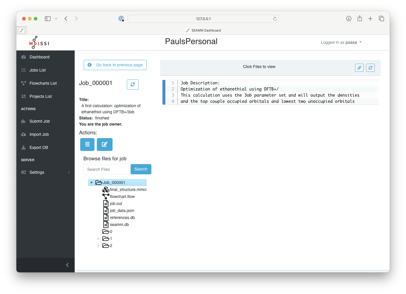
The main page of a job#
The job title appears at the top of the left-pane on the screen followed by further details about the job. The longer job description is in top of the right-pane. There is plenty of space, so feel free to write good descriptions.
Now, click on the final_structure.mmcif file in the directory section:
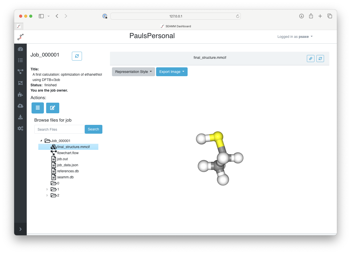
Displaying the final structure#
You can rotate the molecule using the mouse, change its representation through the menu at the top of the screen, or export a screenshot of the current view of the molecule.
Navigate to the job.out file by clicking on it:
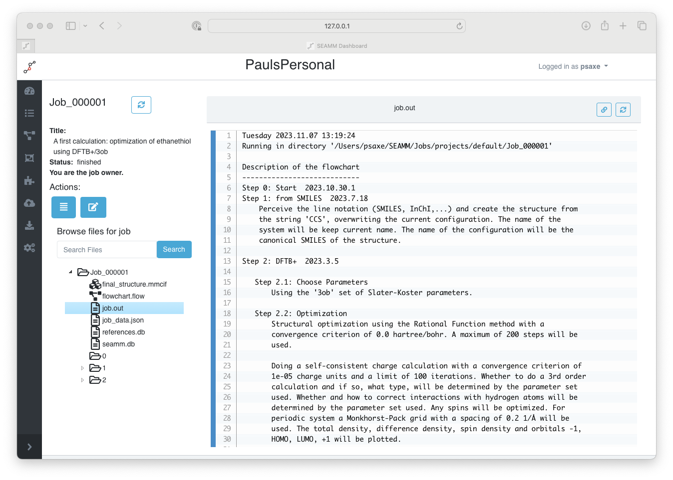
The main output of the job#
This is the main output for our executed job which summarizes its results accompanied by a list of citations at the end. Let us spend some time understanding the information being presented. The first section is always a summary of the job workflow and the steps involved:
Description of the flowchart
----------------------------
  Step 0: Start  2023.10.30.1
  Step 1: from SMILES  2023.7.18
      Perceive the line notation (SMILES, InChI,...) and create the structure from
      the string 'CCS', overwriting the current configuration. The name of the
      system will be keep current name. The name of the configuration will be the
      canonical SMILES of the structure.

  Step 2: DFTB+  2023.3.5

     Step 2.1: Choose Parameters
         Using the '3ob' set of Slater-Koster parameters.

     Step 2.2: Optimization
         Structural optimization using the Rational Function method with a
         convergence criterion of 0.0 hartree/bohr. A maximum of 200 steps will be
         used.

         Doing a self-consistent charge calculation with a convergence criterion of
         1e-05 charge units and a limit of 100 iterations. Whether to do a 3rd order
         calculation and if so, what type, will be determined by the parameter set
         used. Whether and how to correct interactions with hydrogen atoms will be
         determined by the parameter set used. Any spins will be optimized. For
         periodic system a Monkhorst-Pack grid with a spacing of 0.2 1/Å will be
         used. The total density, difference density, spin density and orbitals -1,
         HOMO, LUMO, +1 will be plotted.
This summary is printed before the job actually starts. This is so you can review all
the steps that are going to be executed and check that the job is doing what you
intended. If there is a mistake, you can kill the job, fix the problems, and submit the
job again. You kill the job by checking it in the list of jobs and clicking the
Delete button.
The summary provides the key parameters controlling the calculations. Note that each step also has the version of the code or plug-in used, which is important for reproducing results, or, if a problem is found with a particulalr version, checking whether the results are ok or not.
The second section of the output summarizes the results from the executed flowchart:
Running the flowchart
---------------------
Step 0: Start  2023.10.30.1

Step 1: from SMILES  2023.7.18
    Perceive the line notation (SMILES, InChI,...) and create the structure from
    the string 'CCS', overwriting the current configuration. The name of the
    system will be keep current name. The name of the configuration will be the
    canonical SMILES of the structure.

    Created a molecular structure with 9 atoms.
           System name =
    Configuration name = CCS

Step 2: DFTB+  2023.3.5

    Step 2.1: Choose Parameters
        Using the '3ob' set of Slater-Koster parameters.


    Step 2.2: Optimization
        Structural optimization using the Rational Function method with a
        convergence criterion of 0.0001 E_h/a_0. A maximum of 200 steps will be
        used.

        Doing a self-consistent charge calculation with a convergence criterion of
        1e-05 charge units and a limit of 100 iterations. Whether to do a 3rd order
        calculation and if so, what type, will be determined by the parameter set
        used. Whether and how to correct interactions with hydrogen atoms will be
        determined by the parameter set used. Any spins will be optimized. For
        periodic system a Monkhorst-Pack grid with a spacing of 0.2 1/Å will be
        used. The total density, difference density, spin density and orbitals -1,
        HOMO, LUMO, +1 will be plotted.

        DFTB+ using 1 OpenMP threads for 9 atoms.

        The geometry optimization converged in 46 steps. The last change in
        energy was -1.23222e-10 Eh.


        The total energy is -8.115706 E_h. The charges converged to 0.000002.
        The calculated formation energy is -76.6 kJ/mol for formula C2 H6 S.

        Successfully handled 6 density and orbital cube files.

                   Atomic charges
           +--------+-----------+----------+
           |  Atom  |  Element  |   Charge |
           |--------+-----------+----------|
           |   1    |     C     |    -0.26 |
           |   2    |     C     |    -0.04 |
           |   3    |     S     |    -0.26 |
           |   4    |     H     |     0.09 |
           |   5    |     H     |     0.08 |
           |   6    |     H     |     0.08 |
           |   7    |     H     |     0.08 |
           |   8    |     H     |     0.07 |
           |   9    |     H     |     0.15 |
           +--------+-----------+----------+


Wrote the final structure to 'final_structure.mmcif' for viewing.
This section is identical to the initial summary, but appears more slowly as the job is
running, and also contains a summary of what the step actually did, and key results.
In this example, the FromSMILES step reports the number of atoms in structure and
where it was put. The DFTB+ Optimization provides the total electronic energy,
number of steps for the geometry optimization, and charges on the atoms.
The final section of the output provides references that should be cited regarding the calculations performed:
Primary references:

(1) Jessica Nash and Eliseo Marin-Rimoldi and Mohammad Mostafanejad and Paul
    Saxe. SEAMM: Simulation Environment for Atomistic and Molecular Modeling,
    version 2023.10.30.1; The Molecular Sciences Software Institute (MolSSI):
    Virginia Tech, Blacksburg, VA, USA, https://doi.org/10.5281/zenodo.5153984,
    DOI: 10.5281/zenodo.5153984

(2) O'Boyle, Noel M. and Banck, Michael and James, Craig A. and Morley, Chris
    and Vandermeersch, Tim and Hutchison, Geoffrey R. Open Babel: An open
    chemical toolbox. Journal of Cheminformatics 2011, 3, 33. DOI:
    10.1186/1758-2946-3-33

(3) Hourahine, B.; Aradi, B.; Blum, V.; Bonafé, F.; Buccheri, A.; Camacho, C.;
    Cevallos, C.; Deshaye, M. Y.; Dumitrică, T.; Dominguez, A.; Ehlert, S.;
    Elstner, M.; van der Heide, T.; Hermann, J.; Irle, S.; Kranz, J. J.; Köhler,
    C.; Kowalczyk, T.; Kubař, T.; Lee, I. S.; Lutsker, V.; Maurer, R. J.; Min,
    S. K.; Mitchell, I.; Negre, C.; Niehaus, T. A.; Niklasson, A. M. N.; Page,
    A. J.; Pecchia, A.; Penazzi, G.; Persson, M. P.; Řezáč, J.; Sánchez, C. G.;
    Sternberg, M.; Stöhr, M.; Stuckenberg, F.; Tkatchenko, A.; Yu, V. W.-z.;
    Frauenheim, T. DFTB+, a software package for efficient approximate density
    functional theory based atomistic simulations. The Journal of Chemical
    Physics 2020, 152, 124101. DOI: 10.1063/1.5143190

(4) Gaus, Michael; Lu, Xiya; Elstner, Marcus; Cui, Qiang. Parameterization of
    DFTB3/3OB for Sulfur and Phosphorus for Chemical and Biological
    Applications. Journal of Chemical Theory and Computation 2014, 10,
    1518-1537. DOI: 10.1021/ct401002w

(5) Gaus, Michael; Goez, Albrecht; Elstner, Marcus. Parametrization and
    Benchmark of DFTB3 for Organic Molecules. Journal of Chemical Theory and
    Computation 2013, 9, 338-354. DOI: 10.1021/ct300849w

Secondary references:

(1) Paul Saxe. From Smiles plug-in for SEAMM for creating structures from
    SMILES, version 2023.7.18; The Molecular Sciences Software Institute
    (MolSSI): Virginia Tech, Blacksburg, VA, USA, https://github.com/molssi-
    seamm/from_smiles_step, DOI: 10.5281/zenodo.5159800

(2) Paul Saxe. DFTB+ plug-in for SEAMM, version 2023.3.5; The Molecular Sciences
    Software Institute (MolSSI): Virginia Tech, Blacksburg, VA, USA,
    https://github.com/molssi-seamm/dftbplus_step

Process time: 0:00:02.155739 (2.156 s)
Elapsed time: 0:00:03.721042 (3.721 s)
Tuesday 2023.11.07 13:19:29
The references are divided based on their importance and number of times they are used in the job. For more complicated flowcharts, the number of references can be very large, so this information is useful for preparing the citations in a publication or report.
The references are also stored in a small database file, references.db. Future
versions of SEAMM will provide tools to merge the references from every executed jobs
in a particular project. This will assist users to properly cite the tools that they have
employed to carry out their study.
Examining Details#
The bottom part of the left panel of the results is the directory structure of the job, which mirrors the step numbers in the both the initial summary and detailed results in job.out. In our example, the DFTB+ calculation was the second step in the flowchart and itself had two substeps. If you open the folder for the second step of the flowchart (labeled 2), which is the DFTB+ step, and then the folder 2 inside it, you will see the inputs and outputs from the optimization step:
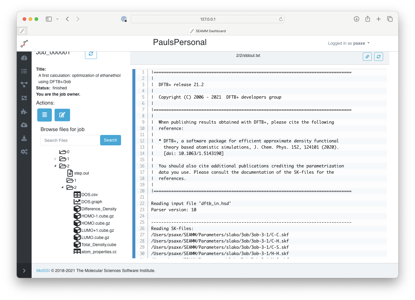
The files for the DFTB+ step#
The main output for DFTB+ is stored in the stdout.txt file which has been selected
in the picture above, so the contents are shown on the right. The input for DFTB+ is
dftb_in.hsd. This is the file that SEAMM created based on the molecule and the
parameters that you set in the DFTB+ GUI. As you can see, it is reasonably complicated,
so SEAMM saved you both work and having to know quite a bit of detail about the
calculation.
Before wrapping up this tutorial, note that the Dashboard will display files in different ways depending on their content and origin. The file list uses difference icons to indicate the type of file. Text files are displayed as text, molecules are represented as three-dimensional structures, volumetric data such as the density and orbitals are shown as 3-D contours, tabular data as sortable tables, and graphs display as such.
For example, if you click on one of the cube files, you will see the corresponding orbital or density. For example, the HOMO:
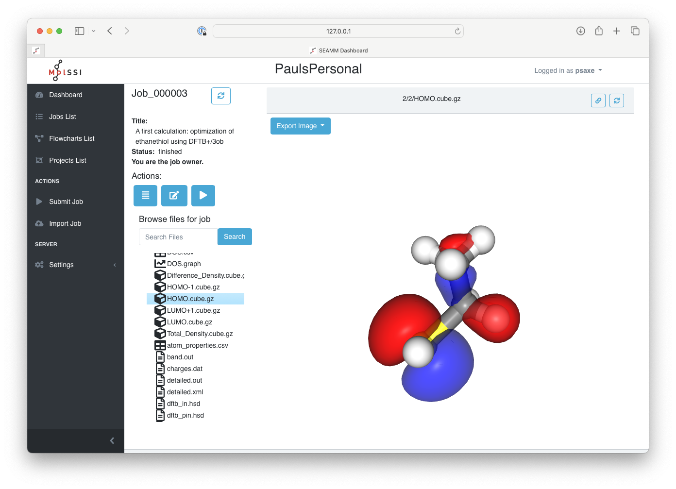
The highest occupied molecular orbital (HOMO)#
Topics Covered#
Accessing the Dashboard
Listing the jobs
Viewing the details of a single job
The parts of
job.out, the main output fileUsing
job.outas a guide to the directory structure of the jobDisplaying various types of files